
Do more with less in MLIP
Reading "Cross-functional transferability in foundation machine learning interatomic potentials"

DOI: 10.1038/s41524-025-01796-y (link)
1. Why Do We Need Machine-Learning Interatomic Potentials?
Modern materials discovery depends on predicting how atoms interact — the potential energy surface that dictates stability, structure, and reactivity.
Density Functional Theory (DFT) has been the workhorse for decades: accurate, quantum-mechanical, but computationally slow. A single DFT calculation can take hours or days, which makes exploring millions of possible materials practically impossible.
Machine-Learning Interatomic Potentials (MLIPs) step in as the fast surrogates. Trained on DFT data, they learn the mapping from atomic environments to total energies and forces, often reproducing DFT accuracy at a cost that is thousands of times cheaper. Foundation models such as CHGNet, M3GNet, and GNoME have shown that one universal potential can simulate crystals, surfaces, and defects across the periodic table.
Yet, these models inherit the limitations of the data they are trained on — and that brings us to the fidelity gap.
2. Why Transfer Learning Is Required
Most existing datasets come from GGA or GGA+U functionals: fast and cheap, but only moderately accurate.
In contrast, r2SCAN and hybrid functionals reach higher fidelity, better capturing strongly bound systems and subtle correlation effects — but at a computational cost roughly ten to a hundred times larger.
That asymmetry creates a classic machine-learning problem:
We have abundant low-fidelity data (millions of GGA structures).
We have scarce high-fidelity data (hundreds of thousands at best).
Training a new MLIP entirely on high-fidelity data would waste the immense knowledge stored in the low-fidelity models. So, we naturally turn to transfer learning — start from the GGA-trained model and fine-tune it with limited r2SCAN data.
Simple in principle. Messy in practice.
3. The Failure of Naive Transfer Learning
Naive transfer learning assumes that the model’s prediction errors are small and smoothly correlated between fidelities.
But when comparing GGA/GGA+U and r2SCAN total energies, the correlation almost vanishes (Pearson ρ ≈ 0.09). The two functionals live on different energy scales, sometimes shifted by tens of eV per atom — far beyond the precision MLIPs aim to learn (≈30 meV/atom).
These shifts are not physical errors. They arise because total DFT energies are defined up to an arbitrary reference — a kind of “zero-point gauge” problem. The energies of r2SCAN and GGA are both valid, but their baselines differ.
If you try to fine-tune the GGA-trained model directly on r2SCAN data, the optimizer sees enormous mismatches. The loss function explodes, gradients become unstable, and performance often becomes worse than training from scratch — a textbook case of negative transfer.
4. The Solution: Change the Reference of Atomic Energy
The key insight from Huang et al. (npj Computational Materials 2025) is that the problem is not the physics, but the energy reference.
In most graph-based MLIPs, the total energy is decomposed as:
Here:
c_{elem} is the vector of element counts in the structure,
E_{AtomRef} are per-element reference energies (fitted by linear regression), and
E_{GNN} is the neural-network correction capturing local bonding.
Sorry, Substack doesn’t have “in-line” math …
If we simply refit these atomic reference energies for r2SCAN, we can align the energy scales before fine-tuning. This tiny adjustment shifts the entire model onto the high-fidelity baseline — just like resetting the zero of potential energy for each element.
Once the scales match, the residuals (the parts the GNN learns) correlate strongly across functionals (ρ ≈ 0.93), and transfer learning becomes smooth and stable.
5. How It Works — A Step-by-Step Illustration
Let’s illustrate with a toy example. Suppose we have three compounds:
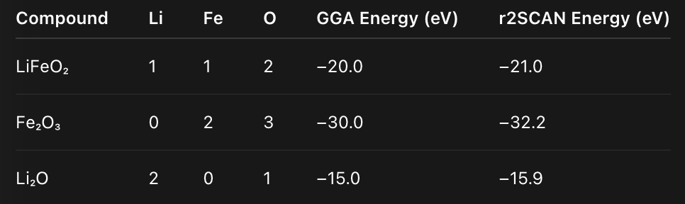
From these, we build a composition matrix A and solve the least-squares equation
This gives per-element reference energies:
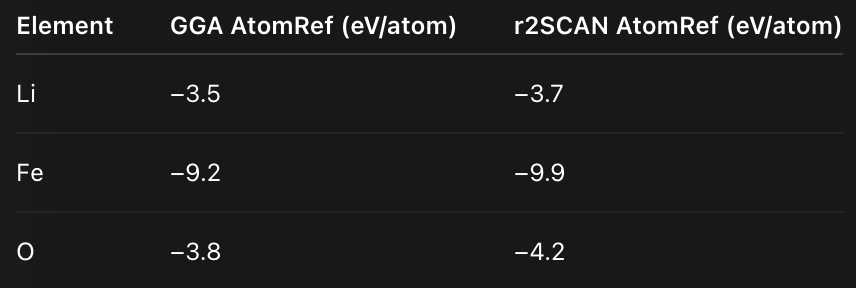
Each element shifts by a few tenths of an eV — small individually, but huge when multiplied across all atoms.
When you substitute E_{AtomRef}^{r2SCAN} into the GGA-trained CHGNet model, all energies move to the correct baseline before training begins. The GNN now starts from a point where predictions differ from r2SCAN by only a few tens of meV, not tens of eV. Fine-tuning becomes efficient and stable.
In practice, this is Method 4 in the paper:
Pre-train CHGNet on GGA/GGA+U.
Compute r2SCAN AtomRef via least-squares fitting.
Replace the GGA AtomRef with the r2SCAN one.
Freeze AtomRef and fine-tune the GNN on r2SCAN data.
The outcome:
Energy MAE = 11.8 meV/atom
Force MAE ≈ 36 meV/Å
10× better data efficiency than training from scratch.
A simple linear correction unlocks full cross-functional transferability.
6. Summary and Outlook: How Much Data Do We Actually Need?
The scaling-law analysis in the paper shows a clean power-law relationship between dataset size and error.
Training from scratch on r2SCAN yields a slope of −0.615 for energy MAE; with transfer learning, the slope becomes −0.301 — shallower, but starting much lower.
That means:
With only 1k r2SCAN structures, transfer learning matches the accuracy of scratch training on 10k structures.
Even at the full 0.24 million-structure dataset, the transfer-learning curve keeps improving — it doesn’t saturate yet.
The message is clear:
Low-fidelity data builds the foundation; high-fidelity data refines it — if and only if you align their energy scales.
This energy-referencing trick might seem mundane, but it’s pivotal. It turns chaotic cross-functional relationships into nearly linear ones and allows us to build truly universal interatomic potentials — models that learn chemistry, not just numbers.
As higher-accuracy DFT datasets (r2SCAN, HSE06, CCSD) continue to grow, the same principle will hold: align the references first, then let the neural network do the fine work. The zero of energy, it turns out, is the key to universality.